Matrix Manual

An introduction into the c4d.Matrix type and some of its associated concepts.

Note

• Cinema 4D uses a left-handed coordinate system.

• All rotations are handled in radians in Cinema 4D.

The Concept of Matrices

A matrix is a rectangular array of numbers. Matrices are organized in row and column vectors where the combined count of of rows and columns is the shape of a matrix. The type Matrix is designed to represent exclusively matrices of the shape 4x4, i.e., four columns and four rows like shown in the image below.

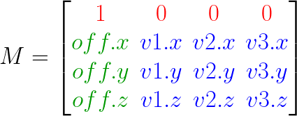
Matrices in general can be used for many things, but the type Matrix has specifically been designed to represent linear transforms. A linear transform, sometimes also linear map (from now on just transform), is a way to represent the mapping from one vector space to another. Another way of looking at that, is to view transforms as a way to express coordinate systems. Due to that, the 4x4 matrix that is represented by the Matrix type, can be split into three different parts.

1. A constant row vector at the top, shown in red in the illustration above, which cannot be changed, due to the fact that Cinema’s transforms do not support projections.

2. A 3x3 sub-matrix in the bottom right corner, shown in blue, which is the basis of the transform and is what quite literally defines the three axis of a three dimensional coordinate system.

3. And an offset vector in the lower part of the first column of the matrix, here shown in green, which as its name implies provides an offset for operation carried out with the transform matrix it is part of.

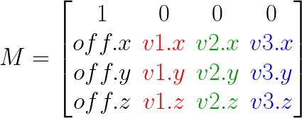
The most important element of these three parts is the 3x3 basis of the transform. It can be split into three three-component vectors, one for each axis of the coordinate system it does represent. These are the basis vectors of the basis which are traditionally labeled as i, j and k or v1, v2 and v3 like Cinema 4D does. This naming convention carries however little meaning and can also be replaced by the respective axis and more common axis labels x, y and z. For each basis vector exists a standard basis vector, namely:

1. (1, 0, 0) for the x-axis (v1 in the terms of the Matrix type).

2. (0, 1, 0) for the y-axis (v2 in the terms of the Matrix type).

3. (0, 0, 1) for the z-axis (v3 in the terms of the Matrix type).

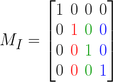
This configuration should be familiar as it reflects the orientations which are usually associated with the respective axes. When the three standard basis vectors in this configuration and an offset that is the zero vector - a vector where all components are zero - form a transform Matrix, that matrix is then called an identity matrix. It is shown in the picture above and is the ‘default state’ for a transform in a certain sense. Which is also why when a Matrix is instantiate without providing any arguments, Cinema will provide us with such an identity matrix.

>>> # Instantiating a matrix with the default arguments will give us the identity matrix.
>>> c4d.Matrix()
Matrix(v1: (1, 0, 0); v2: (0, 1, 0); v3: (0, 0, 1); off: (0, 0, 0))

Carrying out Transforms

The product of a Vector and a Matrix returns the vector operand transfered into the coordinate system represented by the Matrix. For an identity matrix, this will appear as if nothing has happened as the identity matrix maintains the identity of the transformed vector, hence its name.

>>> # Multiplying a point by the identity matrix will give us the same point back.
>>> c4d.Vector(0, 1, 0) * c4d.Matrix()
Vector(0, 1, 0)

When the offset component is provided, all points transformed by that Matrix will be translated by that amount.

>>> # Will return (4, 4, 4), because (1, 2, 3) + (3, 2, 1) = (4, 4, 4)
>>> c4d.Vector(1, 2, 3) * c4d.Matrix(off=c4d.Vector(3, 2, 1))
Vector(4, 4, 4)

One can however provide any combination of all the four components of a Matrix, the offset vector and the three basis vectors v1, v2 and v3, on instantiation. In the example below a Matrix is defined with an x and z axis which are being rotated by 90° counter-clockwise on the z-axis.

Note

A positive rotation in radians goes counter-clockwise, referred to as ‘ccw’ from now on, due to how the circle functions map values. Negative rotations go clockwise, which will be abbreviated as ‘cw’ form now on.

>>> M = c4d.Matrix(v1=c4d.Vector( 0, 1, 0),
                   v2=c4d.Vector(-1, 0, 0))
>>> M
Matrix(v1: (0, 1, 0); v2: (-1, 0, 0); v3: (0, 0, 1); off: (0, 0, 0))

Applying this transform to a Vector will reflect that 90° ccw rotation on the z-axis by rotating the Vector by that amount on that axis.

>>> # Rotates the vector aligned with the axis +y 90° ccw into the position of the axis -x.
>>> c4d.Vector(0, 1, 0) * M
Vector(-1, 0, 0)

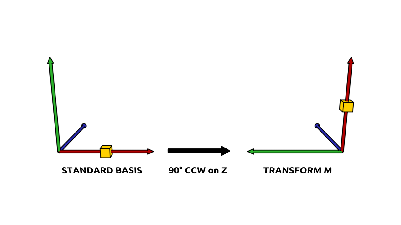
In the picture above the standard basis is shown on the left and the Matrix M defined in the previous example is shown on the right. Also shown is a point in yellow which is rotated with that Matrix M. This demonstrates the idea that a transform is a coordinate system. In a certain sense not the point is being rotated, but the coordinate system around it, since the point is in the same relation to both basis, i.e. coordinate systems.

Aside from this encoding of orientations, transforms also encode scalings. Until now the examples only provided basis vectors of the length of exactly one, i.e., unit vectors. Below is an example which passes vectors for the basis vectors that share the orientation of the standard basis vectors but differ from their length for the x and y axis. The provided v1 has a length of 2, scaling the x component of each vector transformed by that transform by the factor of 2. Similarly, v2 has a length of 0.5, scaling the y-component of vectors transformed by the factor of 0.5.

>>> # A transform oriented like the standard basis, but differing in scale on x and y.
>>> M = c4d.Matrix(v1=c4d.Vector(2, 0, 0),
                   v2=c4d.Vector(0,.5, 0),
                   v2=c4d.Vector(0, 0, 1))
>>> M
Matrix(v1: (2, 0, 0); v2: (0, 0.5, 0); v3: (0, 0, 1); off: (0, 0, 0))

# Multiplying a point with that matrix will give us the scaled point back.
>>> c4d.Vector(2, 3, 0) * M
Vector(4, 1.5, 0)

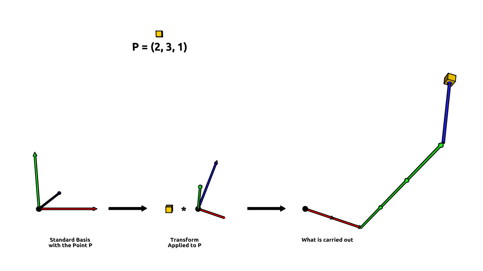
The operation of scaling and rotation can also be combined in a single matrix. As shown in the illustration above, these operations then can be viewed as a combination of the basis vectors, where the components of the transformed point determine the factor with which the basis vectors are scaled. In the illustration above a point P is provided in the world frame with the coordinates (2, 3, 1). Also provided is a transform M. The result of p * M is then equal to p.x * v1 + p.y * v2 + p.z * v3 (ignoring the idea of an offset for now).

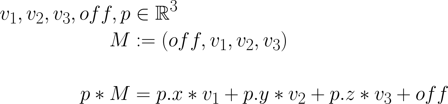
This idea can be formalized with the concept of linear combinations, which is one way of looking at the math being carried out under the hood by Cinema 4D. The little equation shown above is not exactly what is Cinema doing internally, but due to the fact that Matrix type does not support projection transforms, this way of looking at it conveys all the necessary information.

Constructing and Combining Transforms

In the previous examples the basis vectors for the Matrices have always been provided in some form of implied a higher insight on the three dimensional Euclidean vector space, i.e., they assumed the reader somehow knows that (-1, 0, 0) is related to the inverse of the x-axis. This is however not very practical when wanting to construct transforms for arbitrary angles.

Transforms can for once constructed with the helper functions provided in c4d.utils, most notable c4d.utils.MatrixRotX(), c4d.utils.MatrixRotY() and c4d.utils.MatrixRotZ(). When using this way of constructing transforms, one has usually to combine multiple transforms into a single transform by matrix multiplication. It is important to understand that matrix multiplication is not commutative , i.e., M * N does not always yield the same product as N * M in matrix multiplication. The code below demonstrates how to construct a Matrix with these helper functions.

>>> import math

>>> u = c4d.Vector(1, 0, 0)
>>> # A rotation of one quarter pi, i.e., 45°. We will need it since rotations are
>>> # handled in radians in Cinema 4D internally.
>>> quarter_pi = math.pi * .25

>>> # A transform rotating by 45° ccw on the x-axis.
>>> X = c4d.utils.MatrixRotX(quarter_pi)
>>> X
Matrix(v1: (1, 0, 0); v2: (0, 0.707, -0.707); v3: (0, 0.707, 0.707); off: (0, 0, 0))

>>> # A transform rotating by 45° cw on the y-axis.
>>> Y = c4d.utils.MatrixRotY(-quarter_pi)
>>> Y
Matrix(v1: (0.707, 0, -0.707); v2: (0, 1, 0); v3: (0.707, 0, 0.707); off: (0, 0, 0))

>>> # A transform rotating by 45° ccw on the z-axis.
>>> Z = c4d.utils.MatrixRotZ(quarter_pi)
>>> Z
Matrix(v1: (0.707, -0.707, 0); v2: (0.707, 0.707, 0); v3: (0, 0, 1); off: (0, 0, 0))

>>> # The product of the three matrices is a matrix rotating by 45° ccw on x, then 45° cw
>>> # on y and finally by 45° ccw on z.
>>> X * Y * Z
Matrix(v1: (0.5, -0.854, 0.146); v2: (0.5, 0.146, -0.854); v3: (0.707, 0.5, 0.5); off: (0, 0, 0))

>>> # Due to matrix multiplication not being commutative, executing the transforms in a
>>> # different order will yield another matrix product.
>>> Z * Y * X
Matrix(v1: (0.5, -0.5, -0.707); v2: (0.146, 0.854, -0.5); v3: (0.854, 0.146, 0.5); off: (0, 0, 0))

Another way to construct a Matrix is via a provided normal and either a chosen up-vector or an also provided bi-normal or tangent. Below is a code listing which goes through this approach.

"""Example for constructing a transform from a vector.

This example can be run as a script with an object selected. It will orient
that object's z-axis towards (1, 2, 3).
"""

import c4d

EPSILON = 1E-5 # i.e, 0.00001

# A vector provided to us somewhere in code for which we want to construct a
# frame. This could be a vertex normal of a polygon or spline object, the
# delta vector between two object positions or anything else.
normal = c4d.Vector(1, 2, 3)

# First we normalize that input to avoid complications further down the road.
normal = normal.GetNormalized()

# When we are only provided with one vector as a starting point, this only
# does define two of the three degrees of freedom. So we have to make up the
# third one, which is usually done with an up-vector, which is just an
# arbitrary vector we are going to use to construct the matrix. it is however
# often beneficial to choose (0, 1, 0) as that vector, hence its name,
# because we usually orient our world in an up-down fashion and therefor this
# choice will often yield results which *feel* intentional.
up = c4d.Vector(0, 1, 0)

# There is however a problem, we will need to take the cross product of our
# input vector and this up vector. Which will be the zero vector when these
# both vectors are parallel or antiparallel (parallel but facing into
# different directions). So we have to first make sure that does not happen.

# We test with the dot product for the spanned angle. normal * up = 1 will
# mean that the vectors are parallel, -1 will mean that they are antiparallel.
# But due to floating point precision we cannot test directly for that, but
# have to use the EPSILON approach shown below. When our up vector is (anti)
# parallel to the input vector, we simply nudge our up vector a little bit.
up = up if 1. - abs(normal * up) > EPSILON else c4d.Vector(EPSILON, 1, 0)

# Now we simply construct the matrix with the cross-product which will give
# us a vector that is a normal to the plane spanned by the two operands.

# In this case we construct our basis in such way that the input vector
# becomes the z-axis. We could of course also do this differently, this
# form is just very often needed.
z = normal.GetNormalized()

# Now we calculate a temporary x-axis which is orthogonal to both our
# input and up vector.
temp = up.Cross(z)
# With that we can construct the y-axis. Also remember to normalize the
# final axis components, so that we do not introduce unintentional scaling.
y = z.Cross(temp).GetNormalized()
# And finally we have to construct the x-axis. We have to do this so that
# our x axis is orthogonal to both the y and z axis.
x = y.Cross(z).GetNormalized()

# if we wanted to, we could also apply a scaling to our matrix here.

# x *= .5 # scale by the factor of .5 on x.
# y *= 2. # scale by the factor of 2. on x.

# We construct our final matrix.
m = c4d.Matrix(v1=x, v2=y, v3=z)

# if there is a selected object ...
if op is not None:
    # set its global matrix as the one we just constructed ...
    op.SetMg(m)
    # and tell Cinema 4D to update.
    c4d.EventAdd()

Non-Orthogonal Matrices

Until now the examples only defined matrices which have been orthogonal, i.e. matrices, where all the basis vectors span a right angle between each other. This was also reflected by the fact that we constructed a Matrix with the cross product in the previous example to maintain that orthogonal relation. This is however not necessary, we can also define non-orthogonal matrices with the Matrix type:

>>> # A non-orthogonal matrix, the basis vector v2 is not orthogonal to v1,
>>> # instead they span a 45° angle.
>>> M = c4d.Matrix(v1=c4d.Vector(1, 0, 0),
                   v2=c4d.Vector(1, 1, 0),
                   v3=c4d.Vector(0, 0, 1))
>>> M
Matrix(v1: (1, 0, 0); v2: (1, 1, 0); v3: (0, 0, 1); off: (0, 0, 0))

When such a transform is carried out on a Vector, the resulting Vector will be skewed. This a forth form of transformation besides the forms of translation, scale and rotation we already have encountered.

>>> c4d.Vector(0, 10, 0) * M
Vector(10, 10, 0)

There is however something special about this kind of Matrix, once we apply such a skew Matrix to an object, Cinema will silently correct it and bring it into an orthonormal form, i.e., make it an orthogonal matrix, as it otherwise would also skew that object.

>>> # A cube object.
>>> cube = c4d.BaseObject(c4d.Ocube)

>>> # We apply our skewed Matrix from above as the global Matrix to the cube.
>>> m
Matrix(v1: (1, 0, 0); v2: (1, 1, 0); v3: (0, 0, 1); off: (0, 0, 0))
>>> cube.SetMg(m)

>>> # When we read out the global Matrix again, we will see that Cinema has
>>> # forced it into an orthonormal form.

>>> cube.GetMg()
Matrix(v1: (1, 0, 0); v2: (0, 1.414, 0); v3: (0, 0, 1); off: (0, 0, 0))

Objects and Matrices

Matrices are also used to store the position, scale and rotation of objects as shown in the last example. In Cinema 4D, each object has can be represented by two matrices, a global and a local one. These matrices can be accessed with the following methods.

• BaseObject.GetMg() - Returns the transform of the object in the world coordinate system.

• BaseObject.GetMl() - Returns the transform of the object in relation to its parent object.

• BaseObject.SetMg() - Sets the transform of the object in the world coordinate system.

• BaseObject.SetMl() - Sets the transform of the object in relation to its parent object.

>>> # A BaseObject in Cinema 4D.
>>> op
<c4d.BaseObject object called Cube/Cube with ID 5159 at 2725971849536>

>>> # It has a global Matrix attached which defines its transform in world space.
>>> mg = op.GetMg()
Matrix(v1: (0.707, 0, 0.707); v2: (0.707, 0, -0.707); v3: (0, 1, 0); off: (100, 200, 0))

>>> # We just pile on another transform onto that Matrix, in this case just a translation
>>> # by 100 units on the x-axis. The order of operands is in important in this case due
>>> # to the non-commutative nature of matrix multiplication.
>>> newMg = c4d.Matrix(off=c4d.Vector(100, 0, 0)) * mg
>>> newMg
Matrix(v1: (0.707, 0, 0.707); v2: (0.707, 0, -0.707); v3: (0, 1, 0); off: (200, 200, 0))

>>> # We write the matrix back as the new global matrix of the object.
>>> op.SetMg(mg)
>>> # The object parameters will reflect that directly, ...
>>> op[c4d.ID_BASEOBJECT_REL_POSITION]
Vector(200, 200, 0)
>>> # ... but to also reflect our changes in the viewport, we have to tell Cinema 4D to update.
>>> c4d.EventAdd()

The global Matrix of an object is equal to the product of the local matrices of its ancestor objects multiplied with the local transform of the object. So for the following hierarchy:

A
└─B
  └─C

the global Matrix of C is equal to A.GetMl() * B.GetMl() * C.GetMl(). This is however a bit backwards way of looking at it, a more intuitive way of looking at local and global transforms, is probably to view local transforms as the parts of a decomposed a global transform. Global and local coordinate systems can sometimes be a bit tricky to handle, which is why it is often considered to be best practice to carry out as many calculations as possible in the world coordinate system.

Freeze Transformations

For (character) animation it is important that you can define rest poses. Most objects carry all kinds of complicated position, scale and rotation information. Freeze Transformations allow you to ‘freeze’ this information, but reset position/rotation to 0.0 and scale to 1.0. One could achieve the same by adding for every single object in a hierarchy a parent null object. Due to that one can think of Freeze Transformations as ‘virtual null objects’.

All parts of the application that deal with keyframing only access values without the freeze transformation part. This way one can conveniently animate and avoid rotation singularities. The correct routines for animation and keyframing are labeled ‘Rel’. Other parts of the application however, need to get the absolute local position of a target - the position that consists of the frozen and regular matrix. For those purposes one has to use the routines that are labeled ‘Abs’. To clarify, as long as an object has no Freeze transformation assigned - which is always the default case when you create a new object - there is no difference between the ‘Abs’ and ‘Rel’.

Note

BaseObject.GetMl(), BaseObject.SetMl(), BaseObject.GetMg() and BaseObject.SetMg() always include the frozen information, thus are ‘Abs’ versions.

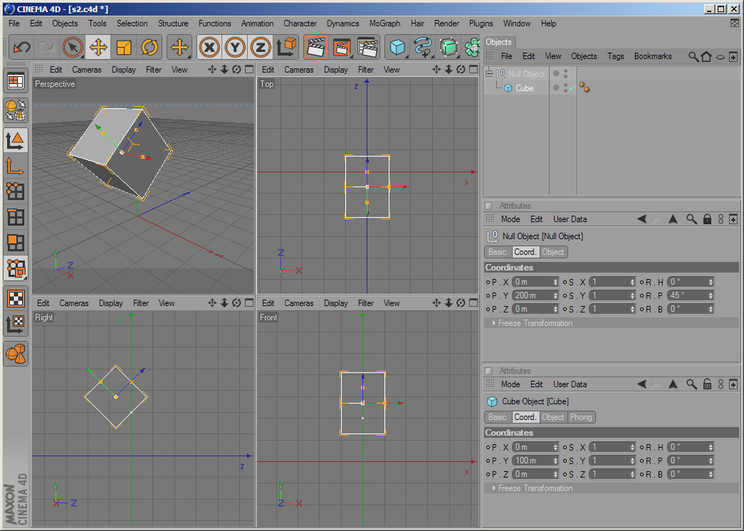
The null object in the picture below has a position of (0, 200, 0) and rotation of (0°, 45°, 0°). The cube has a position of (0, 100, 0). You can see to the left its global position in space.

Now let us try to do the same with one single object:

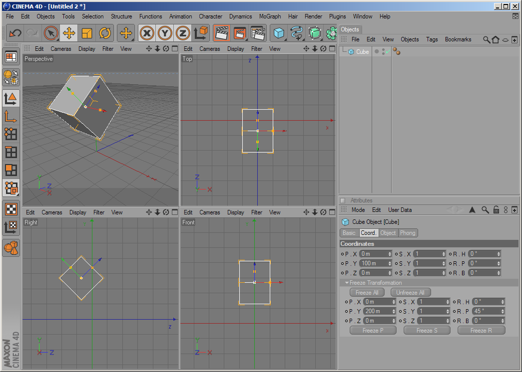
One see that the Null object’s position and rotation have been transferred to the Cube’s frozen position and frozen rotation. The result is exactly the same as before, just without the need for an extra null object. When now BaseObject.GetAbsPos() is called on the cube object, the return value will be (0, 270.711, -70.711). When BaseObject.GetRelPos() is being called however, the return value will be (0, 100, 0). The coordinate manager offers exactly those two display modes: ‘Object (Abs)’ and ‘Object (Rel)’.

As copying position, rotation and scale data from one object to another is much more complex than before there is a new routine BaseObject.CopyMatrixTo() that copies all position, rotation and scale data (including the frozen states) over to another object.

In Cinema 4D the matrix multiplication order for two matrices A and B:

[C] = [A] * [B]

is defined as the rule “A after B”, so the following two lines are equivalent:

transformed_point = original_point * [C]
transformed_point = (original_point * [B]) * [A]

(the original point is first transformed by matrix [B] and then later by [A])

An object’s global matrix is calculated like this:

[Global Matrix] = [Global Matrix of Parent] * [Local Matrix]

or

[Global Matrix] = op.GetUpMg() * op.GetMl()

To calculate the local matrix of an object the formula is:

[Local Matrix] = [Frozen Translation] *
                 [Frozen Rotation] *
                 [Relative Translation] *
                 [Relative Rotation] *
                 [Frozen Scale] *
                 [Relative Scale]

or

[Local Matrix] = MatrixMove(op.GetFrozenPos()) *
                 HPBToMatrix(op.GetFrozenRot()) *
                 MatrixMove(op.GetRelPos()) *
                 HPBToMatrix(op.GetRelRot()) *
                 MatrixScale(op.GetFrozenScale) *
                 MatrixScale(op.GetRelScale())

or equally

[Local Matrix] = MatrixMove(op.GetAbsPos()) * HPBToMatrix(op.GetAbsRot()) * MatrixScale(op.GetAbsScale)

Please note that the both scales are applied at the very beginning, so the local matrix is not the same as [Frozen Matrix] * [Relative Matrix]. This is necessary in order to guarantee that the local matrix always stays a rectangular system.